The Solar Ledger

Introduction

Evaluating the true potential of a plug-in solar system starts with understanding your actual household energy demand. To figure out whether a DIY plug-in solar setup makes sense for my home, I analyzed my electricity usage over a full 12-month period—from August 1, 2025 through July 31, 2026.

While utility billing cycles rarely align perfectly with calendar months, I used a linear regression cost model to overcome this. As discussed in my previous article on building an open data pipeline and cost impact model, this approach lets me calculate energy consumption and estimated costs for any custom date range with high accuracy.

Why Split Usage by 2?

A key technical detail when evaluating plug-in solar is how standard North American residential electrical panels work. Most homes receive 240V split-phase power divided into two separate 120V “legs” or lines. Because standard plug-in solar microinverters plug into a standard 120V wall outlet, they only feed power into one of those two legs.

To estimate how much electricity usage a single-leg solar setup can offset, I divide total household energy consumption by two. Assuming a clean 50/50 balance between Leg 1 and Leg 2 is an approximation, but it is the only practical approach available given that my utility only provides whole-home consumption in 30-minute blocks.

Estimating that each leg represents 50% of energy consumption holds up best during peak summer months, which account for the bulk of my annual grid import. My central air conditioner runs on a 240V circuit, drawing power equally across both legs simultaneously, and it represents roughly half of my summer electricity consumption. The remaining ~50% of summer consumption primarily consists of discrete 120V loads whose phase distribution is unmetered.

In the winter, when the AC is idle, almost all consumption shifts to those 120V circuits. Because I haven’t mapped individual branch circuits to their respective legs, I can't be as confident about how evenly balanced that winter usage really is, but without panel-level monitoring an even split remains the most sensible estimate.

Annual Usage Breakdown & Monthly Highlights

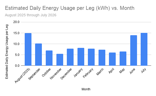
Here is the breakdown of my energy consumption across all 12 months, along with the estimated daily usage per leg:

Month	Daily Energy Usage per Leg (kWh)	Total Energy Usage per Leg (kWh)	Cost per Leg	Effective Rate per kWh
August (2025)	15.0	465.2	$76.99	$0.17
September	10.2	305.8	$52.64	$0.17
October	7.0	216.2	$38.96	$0.18
November	5.5	164.4	$31.05	$0.19
December	7.8	241.8	$42.87	$0.18
January (2026)	8.2	253.6	$44.67	$0.18
February	7.8	217.6	$39.17	$0.18
March	7.4	228.8	$40.88	$0.18
April	6.1	181.5	$33.66	$0.19
May	6.6	203.9	$37.08	$0.18
June	14.1	421.5	$70.32	$0.17
July	15.1	468.6	$77.51	$0.17

Looking at the monthly trends, November 2025 represented the lowest usage month of the year at 328.8 kWh total (an average of 5.5 kWh/day per leg). On the opposite end, July 2026 hit the highest usage peak at 937.2 kWh total (an average of 15.1 kWh/day per leg).

The total estimated cost for the single leg of energy over this 12-month period was $585.77. This figure represents the absolute maximum theoretical savings a plug-in solar system could have achieved under Dominion Energy Virginia's rate structure. Because a standard plug-in solar setup cannot generate enough electricity to fully offset this demand (even if oversized by 25%) this amount sets a firm ceiling on expected cost savings.

Seasonal Trends & HVAC Impact

Energy consumption changes significantly across the seasons due to heating and cooling demands:

• Shoulder Seasons (Fall & Spring): During spring and autumn, my heating and cooling systems stay off most of the time. Opening windows handles temperature control, leading to the lowest electrical demand of the year.
  
• Winter Heating Demand: Because my home uses natural gas for primary heating rather than an electric heat pump, winter electricity demand remains modest. However, daily usage still rises compared to shoulder seasons because the furnace fan requires electric power to circulate warm air.
  
• Summer Peak Demand: Air conditioning drives the largest electricity load by far, doubling or tripling daily usage compared to spring and fall months.

Note: I started charging my EV at my house in June. Charging raised my total electricity usage for June and July but the overall trends for the year remain consistent, I’ve now just raised my baseline electricity usage.

Conclusion & What's Next

By analyzing a full year of energy consumption, I established a clear understanding of the maximum impact a plug-in solar system can have. In the next post, I’ll demonstrate the grid-power offset potential of the previously modeled 1,200 W and 1,500 W systems at a more granular level and the expected payback periods.

Tags: #Solar #PlugIn #Balcony #Modeling

Modeling 1,200W vs. 1,500W in Virginia

When exploring plug-in solar, a natural first question is: How much electricity will this system actually generate every day?

To answer this with mathematical precision rather than marketing guesswork, I modeled daily solar generation for my residence in Fairfax County, Virginia over a full 365-day year (August 2025 to July 2026). Using physics-based modeling and hyper-local historical weather data, here is what the data reveals about plug-in solar generation, the impact of panel “overpaneling,” heat penalties, and potential real-world saving.

1. Regulatory Context: Why the 1,200 W Inverter Cap?

Under Virginia’s plug-in solar law, residential plug-in solar devices up to 1,200 Watts DC per dwelling unit can be connected directly into standard 120V household wall outlets without formal utility pre-approval, interconnection fees, or complex electrical panel upgrades.

However, a solar array with a nameplate capacity of 1,200 W would rarely reach that limit due to weather effects (clouds, heat, or time of year). Commercial installations typically oversize their arrays about 25% to be able to reliably generate the expected amount of energy. Virginia’s plug-in solar law does not allow for oversizing but it’s an interesting analysis to see the extra value you would get from an oversized array with a microinverter that would limit the output to 1,200W.

2. The Modeling Setup: 1,200 W vs. 1,500 W Arrays

Using the physics-based Python pvlib library (implementing NREL’s benchmark PVWatts DC model) combined with 30-minute irradiance, ambient temperature, and wind speed data from the Open-Meteo API for Fairfax County, VA (38.85° N, -77.13° W), I simulated two fixed, South-facing (180° azimuth) arrays tilted at 38.85°:

• Baseline Array: 1,200 W DC nameplate capacity paired with a 1,200 W inverter (95% DC-to-AC efficiency).
  
• Oversized Array: 1,500 W DC nameplate capacity (25% more panel capacity) paired with the same 1,200 W max inverter output limit.

3. Average Daily Generation & Dollar Savings

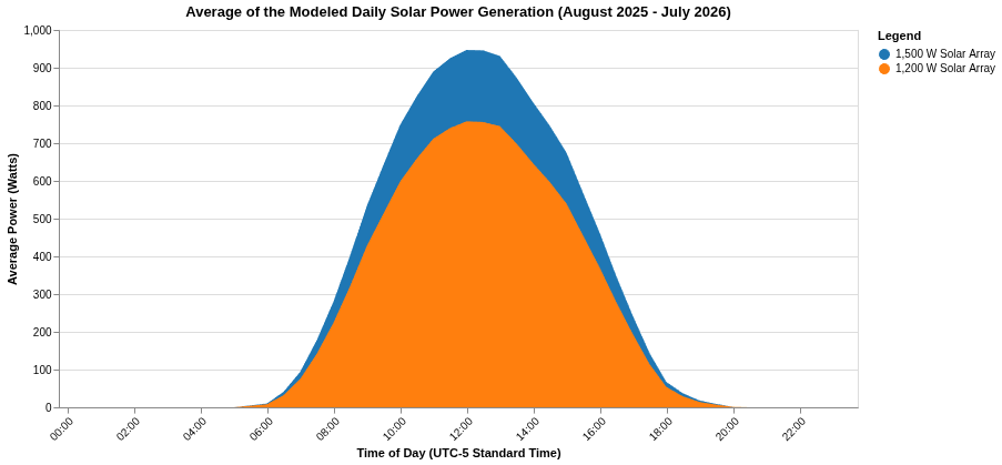
Below is a graph of how much energy each system would produce based on an average of the days across the entire year:

The table below gives greater detail and the expected savings if 100% of the generated, energy displaced electricity that otherwise would have been pulled from the grid.

System Configuration	Raw Daily Generation (kWh)	Daily Output Limited to 1,200 W (kWh)	Energy Lost to Clipping	Estimated Daily Value ($0.18/kWh)	Estimated Annual Value
1,200 W Solar Array	5.344 kWh	5.343 kWh	0.02%	~$0.96 / day	~$350 / year
1,500 W Solar Array	6.683 kWh	6.589 kWh	1.41%	~$1.19 / day	~$432 / year

Clipping occurs when the solar array outputs more power than enough power for the microinverter to produce 1,200 W AC. A legally compliant microinverter would limit the output to 1,200 W (clipping) so that the system remains compliant with the law.

My average cost of electricity is $0.18/kWh. However, this cost depends on total usage. In my county, we have three different categories of costs that scale differently: * Strictly Proportional Charges (generation, transmission, fuel, deferred fuel cost charge, sales and use surcharge, and state/local consumption tax scale linearly with consumption. * Partially Proportional Charges: distribution service charge consists of a fixed monthly customer charge plus a variable per-kWh rate. * Capped Non-Proportional Charges: County utility tax contains a fixed base fee plus a capped variable rate.

The Power of “Overpaneling”

By oversizing the panel array by 25% (1,500 W total panels feeding a 1,200 W max output), the total delivered daily output increases by 23.33% (from 5.34 kWh to 6.59 kWh per day). Even though peak midday generation exceeds the 1,200 W inverter limit on clear days. Based on this average output value, only 1.41% of total potential annual power would be lost to clipping.

4. Hardware & Purchasing Costs: Is Oversizing Worth It?

Retail rigid solar panels (300 W to 400 W nameplate ratings from major manufacturers like Renogy, BougeRV, Aptos, or EcoFlow) typically cost $120 to $180 per panel ($0.40–$0.55 per Watt).

• Baseline 1,200 W Hardware: Four 300 W panels (~$600 total panel cost).
  
• Oversized 1,500 W Hardware: Five 300 W panels (~$750 total panel cost).

Adding one extra 300 W panel costs approximately $150. At $0.18 per kWh, generating an additional 1.25 kWh per day provides $0.225/day ($82.12/year) in extra value. That extra panel pays for itself in under 20 months.

5. High vs. Low Days: The Counterintuitive “Heat Penalty”

Solar production isn't just a function of daylight hours; temperature plays a massive role due to the solar panel temperature coefficient (-0.0047 / °C).

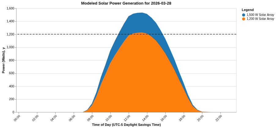
• Clear Spring Day (March 28, 2026 - High Temp 49°F):
  
  • 1,200 W Array Output: 8.96 kWh (clipped)
    
  • 1,500 W Array Output: 10.11 kWh (clipped)
    
  • Cool ambient temperatures keep panel efficiency near maximum, yielding over 10 kWh in a single day!
    

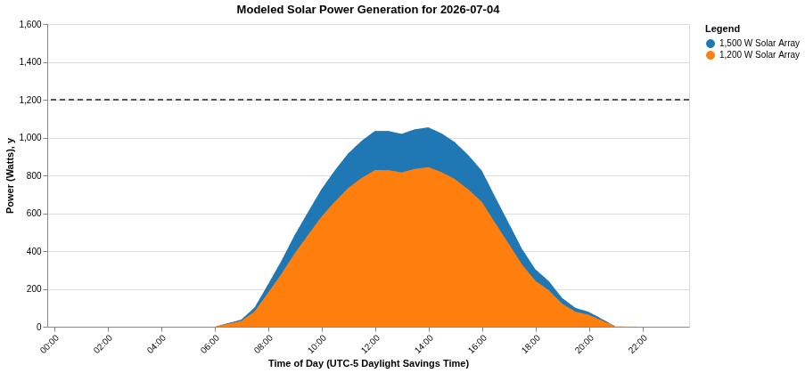
• Hot Summer Day (July 4, 2026 - High Temp 103°F):
  
  • 1,200 W Array Output: 6.70 kWh
    
  • 1,500 W Array Output: 8.37 kWh
    
  • Extreme summer heat derates panel output, and atmospheric haze/humidity reduces solar intensity—producing about 75% of the daily output of a crisp spring day despite longer daylight hours!

6. What's Coming Up Next: Real Household Demand Analysis

Knowing how much power your panels generate on paper is only half the battle. Because plug-in solar operates on a single 120V circuit leg without net metering, any power produced above your home's instantaneous demand flows out to the grid for free.

In my next post, I'll look at real smart meter data from my home! I'll analyze 30-minute interval electrical load profiles across single-phase circuits to calculate exact real-time self-consumption and uncompensated exports. Stay tuned!

Tags: #Solar #PlugIn #Balcony #Modeling

To evaluate the true financial returns of plug-in solar and battery storage, generalized assumptions must be replaced with high-resolution empirical data. Minute-by-minute data would enable excellent modeling, however this requires specialized equipment installed in the breaker box and a dedicated data capture system. Fortunately, most utilities offer 30-minute utility meter interval readings you can download from your account. With this data , plus past bills, meteorological data, and a physics-based photovoltaic (PV) simulation, I was able to create an excellent model of the actual utility power offset and the projected impact to my bill.

1. Data Extraction: Navigating Utility Export Limitations

The utility industry established the Green Button Energy Service Provider Interface (ESPI) XML standard to allow consumers to download energy usage data. However, data collection from my utility revealed two critical limitations in Green Button XML exports:

• UI Restrictions & Date Limits: The customer portal's XML export tool enforces a restriction limiting downloads strictly to the trailing 13 months, blocking access to historical multi-year data.
  
• Low Data Precision: Green Button XML exports round consumption readings to whole integer kilowatt-hours (1 kWh resolution), obscuring subtle household power dynamics.

To overcome this, I chose to build my data pipeline using my utility’s “Download Detailed Data” Excel (.xlsx) export option. This format provides continuous 30-minute interval readings at three decimal places of precision (0.001 kWh). An automated Python ETL script parses these workbooks, aligns intervals chronologically, and ingests them into a local DuckDB time-series database. 

2. Bill Parsing & Tariff Structure Regression

Standard solar calculators assume an average flat electricity rate, but real utility tariffs consist of complex, multi-tiered line items. To model financial savings accurately, I created a Python script to extract the 21 meaningful line items from the monthly PDF bill statements. I used ordinary least squares (OLS) linear regressions with the data to classify fee behavior into three structural categories:

1. Strictly Proportional Charges: Generation, transmission, fuel, deferred fuel cost, sales/use surcharge, and state/local consumption taxes scale linearly down to zero with lower kWh usage.

2. Partially Proportional Charges: Distribution service charges consist of a fixed monthly base customer fee of $11.23 plus a variable per-kWh rate.

3. Capped Non-Proportional Charges: The local utility tax consists of a \$0.60 base fee plus a variable rate capped at a maximum of \$4.00/month.

When solar generation reduces grid energy consumption, fixed customer base fees and tax caps remain untouched while variable supply and distribution rates scale down proportionally.

3. Satellite Solar Irradiance & Performance Modeling

Solar generation potential was derived using historical meteorological data retrieved from the Open-Meteo API for my county. The dataset provides 30-minute resolution Global Horizontal Irradiance (GHI), Direct Normal Irradiance (DNI), Diffuse Horizontal Irradiance (DHI), ambient temperature, and wind speed.

Photovoltaic DC output was calculated using the physics-based PVWatts DC model implemented via Python's pvlib library (utilizing benchmarks established by my favorite National Lab - the National Laboratory of the Rockies, formerly NREL):

• System DC Rating: 1,200, 1,300, 1,400, and 1,500 W
  
• Array Orientation & Tilt: Fixed South-facing (Azimuth \= 180°), 38.85° tilt angle (equal to site latitude)
  
• Temperature Coefficient: -0.0047 / °C
  
• Inverter Conversion Efficiency: 95.0% DC-to-AC
  
• Battery Round-Trip Efficiency: 95.0%
  

4. Interval Simulation & Split-Phase Logic

For each 30-minute block, AC solar generation is calculated:

$$\text{Solar AC (kWh)} = \left(\frac{\text{DC Power (W)} \times 0.5\text{ hrs}}{1000}\right) \times \text{Inverter Efficiency}$$ Net grid energy draw is then evaluated under an assumed 50/50 split-phase load across two 120 V legs (while this is not an ideal assumption, it’s the the best approximation I can make given the data I have available):

• Solar-Only Configuration (Single-Phase Injection): Solar offsets Leg 1 only. Any generation exceeding Leg 1's simultaneous load ($0.5 \times \text{Grid Demand}$) cannot cross phases and flows back to the utility grid uncredited. As a result, the maximum possible power offset is limited to 50% of Grid Demand:

$$\text{Grid Draw} = \max(0, 0.5 \times \text{Grid Demand} – \text{Solar AC}) + 0.5 \times \text{Grid Demand}$$

• Solar + Battery Configuration: A 2.0 kWh modular LiFePO₄ battery buffers excess generation on Leg 1 before it reaches the main service panel, eliminating single-phase export losses and discharging to offset aggregate household demand over time:

$$\text{Grid Draw} = \text{Grid Demand} – (\text{Solar AC} \times \text{Battery Efficiency})$$

Tags: #Solar #PlugIn #Balcony #BatteryStorage #Modeling

Why Online Calculators Lie

Residential solar is undergoing a major structural transformation. Home solar adoption has historically been defined by large-scale rooftop installations requiring steep upfront capital investments, complex municipal permitting, structural engineering assessments, and formal utility interconnection agreements. Today, a new class of accessible technology (plug-in/balcony solar solar) is gaining massive popularity. In Virginia, for example, a recent law will make plug-in solar systems up to 1,200 W DC legal starting January 1, 2027 (the full text of the law can be found on the Virginia Legislative Information System). Rather than requiring hard-wiring into a main breaker panel through a dedicated circuit, these micro-systems plug directly into standard residential AC outlets.

Despite growing consumer interest, evaluating the true financial return of small-scale plug-in systems remains surprisingly difficult. Most web-based solar estimators rely on crude monthly averages and oversimplified financial assumptions that fail to capture the realities of utility rate structures and instantaneous power demand. Standard solar estimators fall victim to three fundamental analytical blind spots:

1. The Naive Proportionality Assumption

Standard calculators typically estimate savings by multiplying total annual solar kWh generation by a single average electricity rate (e.g., $0.18/kWh). In reality, utility bill tariffs are non-linear. Electric bills are composed of fixed monthly customer service charges, fixed administrative fees, step-down tax rates, and capped municipal taxes. Reductions in electricity consumption lower variable energy supply charges, but leave fixed customer base fees entirely untouched.

2. The Interval Simultaneity Problem

Electricity generation and household consumption must match instantaneously in real time. If a 1.2 kW solar array generates 900 Watts of power at 1:00 PM on a sunny afternoon, but household baseload demand is only 300 Watts, the remaining 600 Watts will flow back into the grid. Plug-in solar in the US doesn't allow for net-metering, this excess daytime energy yields zero financial credit.

3. The Split-Phase Injection Blind Spot

Crucially, standard solar models overlook a foundational physical constraint of North American residential electrical architecture: 120V/240V split-phase service. Power is delivered across two separate 120 V legs (Leg 1 and Leg 2). A standard 120 V plug-in solar microinverter connects to a single branch receptacle wired exclusively to one leg. Solar power injected into Leg 1 cannot cross over in real time to offset 120 V loads running on Leg 2. Even if total household demand equals or exceeds instantaneous solar generation, any solar output exceeding Leg 1's isolated load flows straight back through the meter uncredited, while Leg 2 continues drawing full paid power from the grid.

By failing to account for single-phase injection and real-time simultaneity, conventional whole-home analyses severely overestimate the self-consumption of solar-only setups—and consequently drastically undervalue the economic necessity of local battery storage.

Tags: #Solar #PlugIn #Balcony #BatteryStorage

Rigorous data analysis, system architectures, and the business of modern solar.

In my opinion, discussions surrounding solar adoption collapse into two extremes: ideological enthusiasm or vendor sales pitches. Both tend to gloss over the practical engineering constraints and economic analysis that determine whether a system actually delivers value.

The Solar Edge is an independent, data-driven blog focused on unpacking the real-world mechanics and value of solar power. It is fundamentally an analytical working notebook. The goal is to develop a deep, first-principles understanding of distributed energy resources by modeling them openly, documenting edge cases, and confronting the friction points where hardware meets policy.